Advanced Filters: Excel’s Amazing Alternative To Regex
One thing I’ve never understood about Excel is why it doesn’t support regular expressions (which the cool kids call regex). Regex allows you to do advanced sorting and filtering. The SeoTools plugin for Excel supports regex, but it — like most cool resources for Excel — is PC-swim only. For those of us red-headed stepchildren Mac […]
One thing I’ve never understood about Excel is why it doesn’t support regular expressions (which the cool kids call regex). Regex allows you to do advanced sorting and filtering. The SeoTools plugin for Excel supports regex, but it — like most cool resources for Excel — is PC-swim only. For those of us red-headed stepchildren Mac users, that blows.
(Disclaimer: I’m not affiliated with the SeoTools plugin in any way.)
However, as it turns out, Excel offers an alternative to regex that gives you all the same functionality — and is available on all operating systems. They’re called advanced filters. And, they’re actually more flexible than regex and much easier to learn. (If you do want to learn how to leverage regex as a marketer, though, I wrote this post on regex for n00bs last year that makes regex achievable for even the most developer-challenged marketer.)
Some Groundwork
Okay, let’s cover some basics, so we can get to the cool stuff.
First of all, if you’re formatting your data as a table, you’ll already have access to quite a few filters. However, sometimes those filters fall short, especially because Excel doesn’t make the filters sensitive to regex. You have two wildcards to work with:
- *: 0 or more characters (equivalent to .* in regex)
- ?: any one character (equivalent to . in regex)
- ?*: 1 or more characters (equivalent to .+ in regex)
Another benefit to advanced filters over a table (as much as I love tables) is that you can easily copy your filtered data to another location, which can be really handy. If you apply a filter of any kind to a formatted table, you can’t put data on either side of it, or you’ll find some of your rows of data disappearing on you. It would be embarrassing to admit how many times I’ve done that. So we just won’t go there, okay? :)
To illustrate the awesomeness of advanced filters, I downloaded an SEMRush organic keyword report for Hipmunk.com. I’m not affiliated with either of these sites, though I love both of them. I just needed a good dataset to work with. You can download the Excel workbook I use to follow along.
Getting All Set Up
All you need is a dataset that you need filtered. I still format it as a table, but it’s more for aesthetic purposes since applying an advanced filter will strip out your table filters. (You can always reapply them when you’re finished spawning new datasets if you want.)
You’ll find the Advanced Filter option under Data > Sort & Filter > Advanced on a PC, and Data > Filter > Advanced Filter on a Mac. Mac users can also right-click on their table and choose Filter > Advanced Filter from the contextual menu. PC users don’t have that option for some reason.
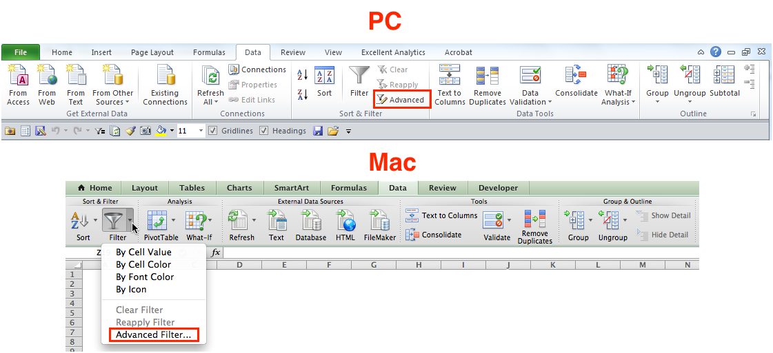
Click for larger image.
Your dataset needs to have headings to use advanced filters, as mine does.
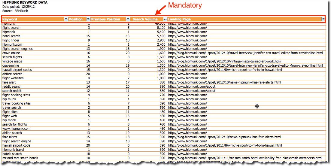
Click for larger image.
A Few Tips
More information about filters is provided below under the headings of key players, headings and multiple criteria.
Key Players
In addition to the wildcards mentioned above, there are a handful of notations you will need to use for your filters:
- =: equality, meaning you want to match whatever comes after it, e.g., =*hipmunk* [include all keywords that contain hipmunk]
- <>: inequality, meaning you want whatever comes after it to be filtered out, e.g., <>https://blog.* [don’t include landing pages from the blog]
- ‘: converts formulas to text when you put it in front of an = sign, e.g., ‘=flight search
- >: greater than, e.g., >500
- >=: greater or equal to, e.g., B4-C4>=3
- <: less than, e.g., C6<D6
- <=: less than or equal to, e.g., <=3
Headings
The way advanced filters work is you copy the headings for the columns you want to filter somewhere outside your dataset. Typically, you’re only going to just need one instance of each heading; but there are times, as you’ll see, where you’ll need to use more than one. You’ll align your heading(s) along the top row, with the criteria immediately below. Don’t worry — I’ll provide you with tons of real-world examples.
Multiple Criteria
There are three basic constructs for multiple criteria:
Or: If you have multiple criteria you need to apply, and either of the criteria could be true, you align these vertically. You can see an example of such a filter from our example dataset below.
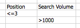
This filter will grab keywords that either rank between 1 and 3 OR have a monthly search volume of greater than 1,000 searches. You could also have multiple “OR” criteria in the same column. If you do, they would all be listed under that column heading.
And: If you have multiple criteria you need to apply and all conditions must be met, you align those horizontally.
![]()
This construct will filter out all non-branded keywords. Remember: those asterisks mean that there may or may not be characters in those locations. The ones between hip and munk (and also monk because people can’t spell) are there to catch all the spellings with spaces that the site ranks for. I could have actually just used *hip* for this site, but marketers will rarely get that lucky in filtering out branded keywords; so, I wanted to demonstrate more the norm. And, if the site ever ranked for something like ship, it would be filtered out.
Both: You can go all fancy pants and have both And and Or conditions.
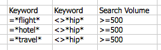
Okay, things are heating up a bit. But this filter simply means I want keywords that include flight, hotel, and travel but don’t contain any branded keywords and have a search volume of at least 500 searches/month.
Note: All I did to get the =*flight,* =*hotel,* and =*travel* to show up as text instead of a formula was put an apostrophe in front of the = sign. Don’t follow the instructions on the Microsoft site. They make it unnecessarily complicated, and I could never get it straight. They say to enter =”=*flight*.” Crazy.
Just this week, as I was preparing this post, I tested using just the apostrophe, and it worked perfectly. If there’s a more convoluted way to do something, Microsoft will find it.
Range: If you want to only see a dataset that falls between a particular range, you would indicate that this way:

This filter captures just keywords that garner between 2,000 and 10,000 searches/month.
Formula: This is what won me about advanced filters. You can actually filter using a formula!
![]()
This formula grabs just the keywords that didn’t move in ranking.
A couple other important notes about using a formula:
- The formula has to resolve to True or False. It can’t return a value
- Don’t include a heading with a formula; just select an empty cell above your formula
- Reference the first cell in your dataset (just below your heading)
- Only use relative cell references, e.g., c4 as opposed to $C$4, which locks your reference
Putting It All Together
Here are the steps you’ll take to filter your data:
Step 1: As mentioned earlier, click any cell inside your dataset, then go to Data > Sort & Filter > Advanced (Mac: Data > Filter > Advanced Filter). This will open the Advanced Filter menu. I’ll use a screenshot from my Mac copy, but all of the options are identical in the PC version. Shockerz.
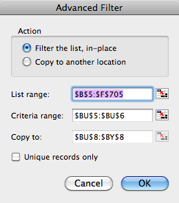
Step 2: Decide if you want to filter the data in place or copy to another location. I usually copy to a new location to keep my original dataset unsullied, but to each his own.
Step 3: For the List Range, by default, Excel selects the entire dataset. You can change that and just select the columns you want. Alternatively, you can type just the headings you want below your criteria and select those cells in the Copy To field, and Excel will only return those columns. I include an example in the Excel workbook you can download, with a green text box with a full explanation.
Step 4: For the Criteria Range, simply click inside the field and select the cells with your criteria. If you want to collapse the menu, just click on range selector to the right of the field and select the cells you want. But you don’t have to collapse the menu to select the cells you need.
Step 5: If you’ve selected Copy to another location at the top of the menu, you can use this field to determine where you want to paste your filtered dataset. You can either choose a single cell, which will become the top-left cell in your dataset, or select pre-typed headings to restrict which columns are copied over.
Step 6: Decide if you just want unique records. Sadly, this is all most people use this amazing filter for — myself included — up until a couple months ago!
Step 7: Click OK, and go retrieve your data.
Step 8: If you filtered your data in place, you can clear your filter, but only if you’re on a PC. It’s due north of the Advanced option. Mac offers this option, but it’s broken … which is another good reason to copy to a new location. If you want to clear the filter, you need to press Command-Z to undo or click a heading cell and choose Filter.
Tons Of Examples
Below are snapshots of the examples I include in the download.
| CRITERIA | SCREENSHOT | EXPLANATION |
| non-branded keywords | link | <> means does not contain |
| keywords ranking on the first page of Google | link | Keyword and Position headings were typed ahead of time to restrict the columns that got copied over |
| keywords with search volumes between 2,000 and 10,000 | link | to get a range, just copy the heading twice and put your lower and upper range in each cell below |
| keywords that garner at least 500 searches/month and contain flight, hotel, or travel but exclude branded keywords | link | if you look inside one of the flight, hotel, or travel cells you’ll see a hyphen in front of the = |
| keywords that get at least 500 searches/month and point to the hipmunk.com blog | link | just like the example directly above, an apostrophe was added to convert the formula to text (shown in screenshot) |
| keywords that are in the top three positions OR get more than 1,000 searches/month | link | it’s okay to have blank cells in the Criteria Range if it’s an OR criteria |
| keywords that contain at least one character before the keyword search | link | the combination of ?* requires at least one character but could contain more (equivalent to .+ in regex) |
| keywords that didn’t move in ranking | you must leave the heading cell above the formula blank AND select it in the Criteria Range | |
| keywords that moved up in ranking | link | self-explanatory |
| keywords that dropped 3 or more rankings | link | when I created the filter I was getting a lot of false positives because SEMRush assigns non-ranking keywords a 0, so I added a condition that the previous rank couldn’t = 0 and joined the two conditions with an AND function |
| get the top 10 keywords by search volume | link | this says, “give me the top 10 most searched keywords” – as indicated by the LARGE function |
Final Tips
There are a few gotchas with advanced filters. As long as you’re aware of them, you should avoid unpleasant surprises.
- If you accidentally include blank cells at the bottom of your criteria range, you will cancel out your criteria because Excel treats blank cells as wildcards that include everything.
- If you want to copy your range to a new worksheet, you need to start the process on the new sheet and just reference the original dataset. Excel won’t let you start on the sheet where your dataset is and select a new worksheet for the Copy To range.
- If you filter your data in place, you can’t have more than one table on a worksheet with advanced filters applied. When you apply filters to the second one, you’ll lose the filters on your original table.
- As mentioned in the post, Clear is broken in Excel 2011 for Mac — at least for me. Let me know in the comments if it works for you! You’ll have to use Command-Z to clear the filter or select the heading and choose Filter. Ironically, this causes Excel to short circuit, and it drops your advanced filter.
- If you have a list of values you need to filter out of your dataset (like I did just last week), I recommend first concatenating your list with <> (learn how), then using Copy > Paste Special > Transpose to get your list running horizontally across your sheet.
Idea For Advanced Excel Users
If you wanted a dynamic filter, you could create drop-down menus with data validation (learn how for 2010 and 2011), and use those values to generate your filters. You’ll still have to run the filter; it won’t run automatically when you select a new option.
However, you could create a simple macro to run the filter (2010/2011) and assign it to a keyboard shortcut or image (2010/2011). Personally, I’d go with the image. I’m not a graphic designer, but here’s one you can use, if you’d like.

If you take the time to play with advanced filters, I think you’ll fall in love with them the way I did because of their simplicity yet unparalleled power.
Opinions expressed in this article are those of the guest author and not necessarily Search Engine Land. Staff authors are listed here.
Related stories
New on Search Engine Land
About the author