An experiment in trying to predict Google rankings
In late 2015, JR Oakes and his colleagues undertook an experiment to attempt to predict Google ranking for a given webpage using machine learning. What follows are their findings, which they wanted to share with the SEO community.

Machine learning is quickly becoming an indispensable tool for many large companies. Everyone has, for sure, heard about Google’s AI algorithm beating the World Champion in Go, as well as technologies like RankBrain, but machine learning does not have to be a mystical subject relegated to the domain of math researchers. There are many approachable libraries and technologies that show promise of being very useful to any industry that has data to play with.
Machine learning also has the ability to turn traditional website marketing and SEO on its head. Late last year, my colleagues and I (rather naively) began an experiment in which we threw several popular machine learning algorithms at the task of predicting ranking in Google. We ended up with an assembly that achieved 41 percent true positive and 41 percent true negative on our data set.
In the following paragraphs, I will take you through our experiment, and I will also discuss a few important libraries and technologies that are important for SEOs to begin understanding.
Our experiment
Toward the end of 2015, we started hearing more and more about machine learning and its promise to make use of large amounts of data. The more we dug in, the more technical it became, and it quickly became clear that it would be helpful to have someone help us navigate this world.
About that time, we came across a brilliant data scientist from Brazil named Alejandro Simkievich. The interesting thing to us about Simkievich was that he was working in the area of search relevance and conversion rate optimization (CRO) and placing very well for important Kaggle competitions. (For those of you not familiar, Kaggle is a website that hosts machine learning competitions for groups of data scientists and machine learning enthusiasts.)
Simkievich is the owner of Statec, a data science/machine learning consulting company, with clients in the consumer goods, automotive, marketing and internet sectors. Lots of Statec’s work had been focused on assessing the relevance of e-commerce search engines. Working together seemed a natural fit, since we are obsessed with using data to help with decision-making for SEO.
We like to set big hairy goals, so we decided to see if we could use the data available from scraping, rank trackers, link tools and a few more tools, to see if we could create features that would allow us to predict the rank of a webpage. While we knew going in that the likelihood of pulling it off was very low, we still pushed ahead for the opportunity for an amazing win, as well as the chance to learn some really interesting technology.
The data
Fundamentally, machine learning is using computer programs to take data and transform it in a way that provides something valuable in return. “Transform” is a very loosely applied word, in that it doesn’t quite do justice to all that is involved, but it was selected for the ease of understanding. The point here is that all machine learning begins with some type of input data.
(Note: There are many tutorials and courses freely available that do a very good job of covering the basics of machine learning, so we will not do that here. If you are interested in learning more, Andrew Ng has an excellent free class on Coursera here.)
The bottom line is that we had to find data that we could use to train a machine learning model. At this point, we didn’t know exactly what would be useful, so we used a kitchen-sink approach and grabbed as many features as we could think of. GetStat and Majestic were invaluable in supplying much of the base data, and we built a crawler to capture everything else.
Our goal was to end up with enough data to successfully train a model (more on this later), and this meant a lot of data. For the first model, we had about 200,000 observations (rows) and 54 attributes (columns).
A little background
As I said before, I am not going to go into a lot of detail about machine learning, but it is important to grasp a few points to understand the next section. In total, much of the machine learning work today deals with regression, classification and clustering algorithms. I will define the first two here, as they were relevant to our project.
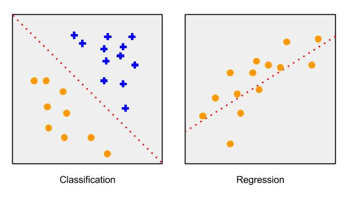
- Regression algorithms are normally useful for predicting a single number. If you needed to create an algorithm that predicted a stock price based on features of stocks, you would select this type of model. These are called continuous variables.
- Classification algorithms are used to predict a member of a class of possible answers. This could be a simple “yes or no” classification, or “red, green or blue.” If you needed to predict whether an unknown person was male or female from features, you would select this type of model. These are called discrete variables.
Machine learning is a very technical space right now, and much of the cutting-edge work requires familiarity with linear algebra, calculus, mathematical notation and programming languages like Python. One of the items that helped me understand the overall flow at an approachable level, though, was to think of machine learning models as applying weights to the features in the data you give it. The more important the feature, the stronger the weight.
When you read about “training models,” it is helpful to visualize a string connected through the model to each weight, and as the model makes a guess, a cost function is used to tell you how wrong the guess was and to gently, or sternly, pull the string in the direction of the right answer, correcting all the weights.
The part below gets a bit technical with terminology, so if it is too much for you, feel free to skip to the results and takeaways in the final section.
Tackling Google rankings
Now that we had the data, we tried several approaches to the problem of predicting the Google ranking of each webpage.
Initially, we used a regression algorithm. That is, we sought to predict the exact ranking of a site for a given search term (e.g., a site will rank X for search term Y), but after a few weeks, we realized that the task was too difficult. First, a ranking is by definition a characteristic of a site relative to other sites, not an intrinsic characteristic of the site (as, for example, word count). Since it was impossible for us to feed our algorithm with all sites ranked for a given search term, we reformulated the problem.
We realized that, in terms of Google ranking, what matters most is whether a given site ends up on the first page for a given search term. Thus, we re-framed the problem: What if we try to predict whether a site will end up in the top 10 sites ranked by Google for a certain search term? We chose top 10 because, as they say, you can hide a dead body on page two!
From that standpoint, the problem turns into a binary (yes or no) classification problem, where we have only two classes: a) the site is a top 10 site, or b) the site is not a top 10 site. Furthermore, instead of making a binary prediction, we decided to predict the probability that a given site belongs to each class.
Later, to force ourselves to make a clear-cut decision, we decided on a threshold above which we predict that a site will be top 10. For example, if we predict that the threshold is 0.85, then if we predict that the probability of a site being in the top 10 is higher than 0.85, we go ahead and predict that the site will be in the top 10.
To measure the performance of the algorithm, we decided to use a confusion matrix.
The following chart provides an overview of the entire process.
Cleaning the data
We used a data set of 200,000 records, including roughly 2,000 different keywords/search terms.
In general, we can group the attributes we used into three categories:
- Numerical features
- Categorical variables
- Text features
Numerical features are those that can take on any number within an infinite or finite interval. Some of the numerical features we used are ease of read, grade level, text length, average number of words per sentence, URL length, website load time, number of domains referring to website, number of .edu domains referring to website, number of .gov domains referring to website, Trust Flow for a number of topics, Citation Flow, Facebook shares, LinkedIn shares and Google shares. We applied a standard scalar (multiplier) to these features to center them around the mean, but other than that, they require no further preprocessing.
A categorical variable is one which can take on a limited number of values, with each value representing a different group or category. The categorical variables we used include most frequent keywords, as well as locations and organizations throughout the site, in addition to topics for which the website is trusted. Preprocessing for these features included turning them into numerical labels and subsequent one-hot encoding.
Text features are obviously composed of text. They include search term, website content, title, meta-description, anchor text, headers (H3, H2, H1) and others.
It is important to highlight that there is not a clear-cut difference between some categorical attributes (e.g., organizations mentioned on the site) and text, and some attributes indeed switched from one category to the other in different models.
Feature engineering
We engineered additional features, which have correlation with rank.
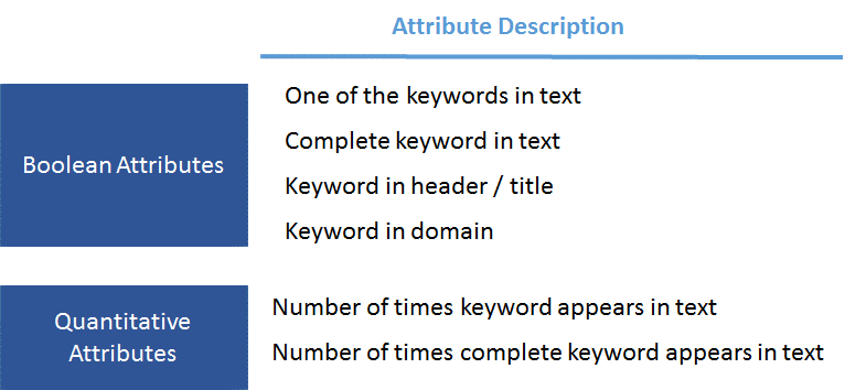
Most of these features are Boolean (true or false), but some are numerical. An example of a Boolean feature is the exact search term included on the website text, whereas a numerical feature would be how many of the tokens in the search term are included in the website text.
Below are some of the features we engineered.
Run TF-IDF
To pre-process the text features, we used the TF-IDF algorithm (term-frequency, inverse document frequency). This algorithm views every instance as a document and the entire set of instances as a corpus. Then, it assigns a score to each term, where the more frequent the term is in the document and the less frequent it is in the corpus, the higher the score.
We tried two TF-IDF approaches, with slightly different results depending on the model. The first approach consisted of concatenating all the text features first and then applying the TF-IDF algorithm (i.e., the concatenation of all text columns of a single instance becomes the document, and the set of all such instances becomes the corpus). The second approach consisted of applying the TF-IDF algorithm separately to each feature (i.e., every individual column is a corpus), and then concatenating the resulting arrays.
The resulting array after TF-IDF is very sparse (most columns for a given instance are zero), so we applied dimensionality reduction (single value decomposition) to reduce the number of attributes/columns.
The final step was to concatenate all resulting columns from all feature categories into an array. This we did after applying all the steps above (cleaning the features, turning the categorical features into labels and performing one-hot encoding on the labels, applying TF-IDF to the text features and scaling all the features to center them around the mean).
Models and ensembles
Having obtained and concatenated all the features, we ran a number of different algorithms on them. The algorithms that showed the most promise are gradient boosting classifier, ridge classifier and a two-layer neural network.
Finally, we assembled the model results using simple averages, and thus we saw some additional gains as different models tend to have different biases.
Optimizing the threshold
The last step was to decide on a threshold to turn probability estimations into binary predictions (“yes, we predict this site will be top 10 in Google” or “no, we predict this site will not be top 10 in Google”). For that, we optimized a cross-validation set and then used the obtained threshold on a test set.
Results
The metric we thought would be the most representative to measure the efficacy of the model is a confusion matrix. A confusion matrix is a table that is often used to describe the performance of a classification model (or “classifier”) on a set of test data for which the true values are known.
I am sure you have heard the saying that “a broken clock is right twice a day.” With 100 results for every keyword, a random guess would correctly predict “not in top 10” 90 percent of the time. The confusion matrix ensures the accuracy of both positive and negative answers. We obtained roughly a 41-percent true positive and 41-percent true negative in our best model.
Another way of visualizing the effectiveness of the model is by using an ROC curve. An ROC Curve is “a graphical plot that illustrates the performance of a binary classifier system as its discrimination threshold is varied. The curve is created by plotting the true positive rate (TPR) against the false positive rate (FPR) at various threshold settings.” The non-linear models used in the ensemble were XGBoost and a neural network. The linear model was logistic regression. The ensemble plot indicated a combination of the linear and non-linear models.
XGBoost is short for “Extreme Gradient Boosting,” with gradient boosting being “a machine learning technique for regression and classification problems, which produces a prediction model in the form of an ensemble of weak prediction models, typically decision trees.”
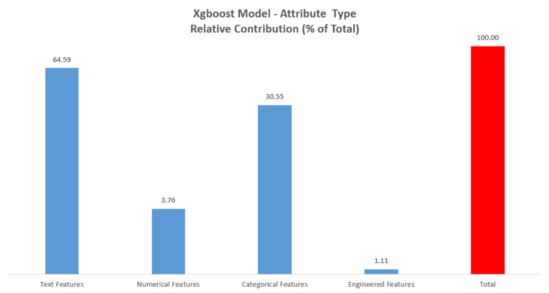
The chart below shows the relative contribution of the feature categories to the accuracy of the final prediction of this model. Unlike neural networks, XGBoost, along with certain other models, allow you to easily peek into the model to tell the relative predictive weight that particular features hold.
We were quite impressed that we were able to build a model that showed predictive power from the features that we had given it. We were very nervous that our limitation of features would lead to the utter fruitlessness of this project. Ideally, we would have a way to crawl an entire site to gain overall relevance. Perhaps we could gather data on the number of Google reviews a business had. We also understood that Google has much better data on links and citations than we could ever hope to gather.
What we learned
Machine learning is a very powerful tool that can be used even if you do not understand fully the complexity of how it works. I have read many articles about RankBrain and the inability of engineers to understand how it works. This is part of the magic and beauty of machine learning. Similar to the process of evolution, in which life gains different features and some live and some die, the process of machine learning finds the way to the answer instead of being given it.
While we were happy with the results of our first models, it is important to understand that this was trained on a relatively small sample compared to the immense size of the internet. One of the key goals in building any kind of machine learning tool is the idea of generalization and operating effectively on data that has never been seen before. We are currently testing our model on new queries and will continue to refine.
The largest takeaway for me in this project was just starting to get a grasp on the immense value that machine learning has for our industry. A few of the ways I see it impacting SEO are:
- Text generation, summarization and categorization. Think about smart excerpts for content and websites that potentially self-organize based on classification.
- Never having to write another ALT parameter (See below).
- New ways of looking at user behavior and classification/scoring of visitors.
- Integration of new ways of navigating websites using speech and smart Q&A style content/product/recommendation systems.
- Entirely new ways of mining analytics and crawled data to give insights into visitors, sessions, trends and potentially visibility.
- Much smarter tools in distribution of ad channels to relevant users.
This project was more about learning for us rather than accomplishing a holy grail (of sorts). Much like the advice I give to new developers (“the best learning happens while doing”), it is important to get your hands dirty and start training. You will learn to gather, clean and organize data, and you’ll familiarize yourself with the ins and outs of various machine learning tools.
Much of this is familiar to more technical SEOs, but the industry also is developing tools to help those who are not as technically inclined. I have compiled a few resources below that are of interest in understanding this space.
Recent technologies of interest
It is important to understand that the gross majority of machine learning is not about building a human-level AI, but rather about using data to solve real problems. Below are a few examples of recent ways this is happening.
NeuralTalk2
NeuralTalk2 is a Torch model by Andrej Karpathy for generating natural language descriptions of given images. Imagine never having to write another ALT parameter again and having a machine do it for you. Facebook is already incorporating this technology.
Microsoft Bots and Alexa
Researchers are mastering speech processing and are starting to be able to understand the meaning behind words (given their context). This has deep implications to traditional websites in how information is accessed. Instead of navigation and search, the website could have a conversation with your visitors. In the instance of Alexa, there is no website at all, just the conversation.
Natural language processing
There is a tremendous amount of work going on right now in the realm of translation and content semantics. It goes far beyond traditional Markov chains and n-gram representations of text. Machines are showing the initial hints of abilities to summarize and generate text across domains. “The Unreasonable Effectiveness of Recurrent Neural Networks” is a great post from last year that gives a glimpse of what is possible here.
Home Depot search relevance competition
Home Depot recently sponsored an open competition on Kaggle to predict the relevance of their search results to the visitor’s query. You can see some of the process behind the winning entries on this thread.
How to get started with machine learning
Because we, as search marketers, live in a world of data, it is important for us to understand new technologies that allow us to make better decisions in our work. There are many places where machine learning can help our understanding, from better knowing the intent of our users to which site behaviors drive which actions.
For those of you who are interested in machine learning but are overwhelmed with the complexity, I would recommend Data Science Dojo. There are simple tutorials using Microsoft’s Machine Learning Studio that are very approachable to newbies. This also means that you do not have to learn to code prior to building your first models.
If you are interested in more powerful customized models and are not afraid of a bit of code, I would probably start with listening to this lecture by Justin Johnson at Stanford, as it goes through the four most common libraries. A good understanding of Python (and perhaps R) is necessary to do any work of merit. Christopher Olah has a pretty great blog that covers a lot of interesting topics involving data science.
Finally, Github is your friend. I find myself looking through recent repos added to see the incredibly interesting projects people are working on. In many cases, data is readily available, and there are pretrained models that perform certain tasks very well. Looking around and becoming familiar with the possibilities will give you some perspective into this amazing field.
Contributing authors are invited to create content for Search Engine Land and are chosen for their expertise and contribution to the search community. Our contributors work under the oversight of the editorial staff and contributions are checked for quality and relevance to our readers. The opinions they express are their own.
Related stories
New on Search Engine Land


