Build SEO seasonality projections with Google Trends in Python
Here's how you can use Python and some very basic Excel functions to build your SEO traffic goals.
Roadmapping season is upon us and, if you’re an in-house SEO like me, that means it’s time to set your FY20 goals for the SEO channel. To set realistic goals, we first need to understand how much traffic we can reasonably drive from SEO this year. To figure this out, we must first answer a few questions:
- How much traffic are we currently driving from SEO?
- If we only take seasonality into account, how much traffic will we drive this year?
- What impact do we expect from the projects on our roadmap?
This article will help answer some of these questions and tie it all together to set your SEO traffic goal using Python and some very basic Excel functions.
How much traffic are we currently driving from SEO?
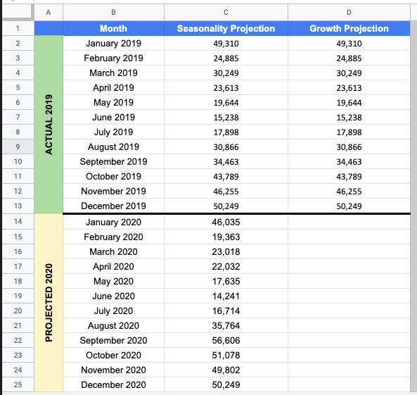
Export monthly traffic for the past year from your analytics platform (Google Analytics or Adobe Analytics). Feel free to use whichever metric you think is best. This can be users, visits, sessions, entrances, unique visitors or a different metric that you use. I recommend using whichever metric is most indicative of search behavior. I personally believe that metric is entry visits/entrances from SEO because a user can enter from search multiple times and we want to capture each entrance. Feel free to use whichever metric is your source of truth.
The data should be formatted similar to the table below:

How much traffic will we drive if nothing changes?
This question is generally the hardest to answer. In the past, I’ve seen some people use traffic patterns from prior years to project seasonality but if you’re on any sort of growth trajectory – which I hope you are – this won’t work for you. I recommend an alternative solution: a seasonality index built with Google Trends data.
Google Trends has a wealth of information about search demand. Google Search Console has a wealth of information about the searches that drive traffic to your website. Connect the two and watch the magic happen.
Step 1: Export Google Search Console Data
Navigate to the search performance tab in Search Console. Change the date range to include the last full year. For example: January 1, 2019 – December 31, 2019. Next, sort the queries by clicks so the top-performing keywords are at the top. Finally, export the top 1000 queries to a .csv file.
Note: if you’d like to be more thorough, you can use Google Data Studio or the Search Console API to export all queries for your site.
Step 2: Collect Google Trends Data
A seasonality index is a forecasting tool used to determine demand for certain products or, in this case, search terms in a given market over the course of a typical year. Google Trends is a powerful tool that leverages the data collected by Google Search to quantify interest for a particular search term over time. We will use the past 5 years of Google Trends interest data to predict future interest over the next year in one-week spans.
Since we want this index to be indicative of the seasonal pattern for traffic to our website, we’ll be basing it on the top-performing keywords for our website that we exported from Search Console in step 1. We’ll also be building this index using PyTrends in Python to remove as much manual work as possible.
PyTrends is a pseudo-API (not supported by Google) for Google Trends that allows us to pull data for large amounts of keywords in an automated fashion. I’ve set up a Google Colab notebook that can be used for this example.
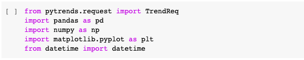
First, we’ll install the required modules to run our code.

Next, well import the modules into our Colab notebook.
We’ll require two functions to create our seasonality index. The first, getTrends, will take a keyword and a dictionary object as parameters. This function will call the Google Trends API and append the data to a list stored in the dictionary object using the dates as a key. The second function, average, will be used to calculate the average interest for each date in the dictionary.

Next, we’ll import our dataset of keywords from Search Console. This can be very confusing in Google Colab so I’ve tried to make it as simple as possible. Follow these steps:
- Upload your CSV file to Google Drive
- Right click on the file, click “Get Shareable Link” and copy the link.
- Replace the link in the code with the link to your file.
- Run the code. The first time it runs, you’ll be asked to authorize Google Drive access by navigating to an authorization page and logging in with your Google account. It will then give you an authorization code. Copy the code and paste it in the box that appears after running the code and hit enter.
We’ll then convert your CSV file to a Pandas DataFrame.

Once we’ve imported our keyword data, we’ll convert the Query column to a list object called keywords. We’ll create an empty dictionary object called data. This is where we will store the Google Trends data. Finally, we’ll iterate over the keyword list to get Google Trends data for each keyword and store it in the data dictionary.

Quick note: Since PyTrends is not an official or Google-supported API, you can run into trouble in this step. I’ve found it best to limit the keyword list to the top 250 queries. Some other steps you can take (which I won’t touch on in this article) are using proxies or adding some random delays in the loop to decrease the chances of being blocked by Google.
Once we’ve collected all of our Google Trends data, we’ll then calculate average interest over time.
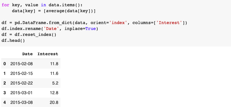
At this point, it can be helpful to plot the results using a time series. We’ll do this using matplotlib.
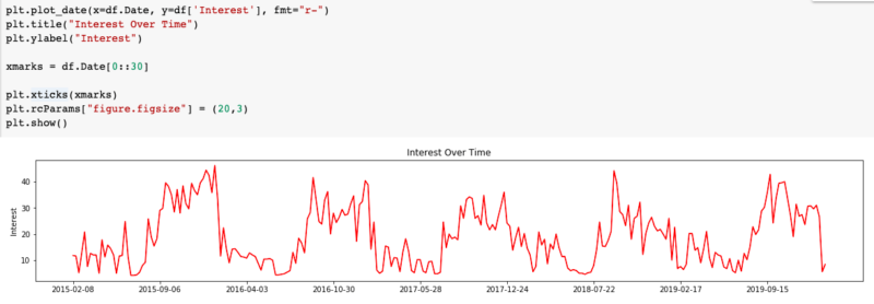
Use this step to verify that the data matches your expectations. Since we’re using NFL teams as our keywords in this example, you’ll notice that the interest peaks during the NFL season and drops off during the off-season. This is what we would expect to happen.
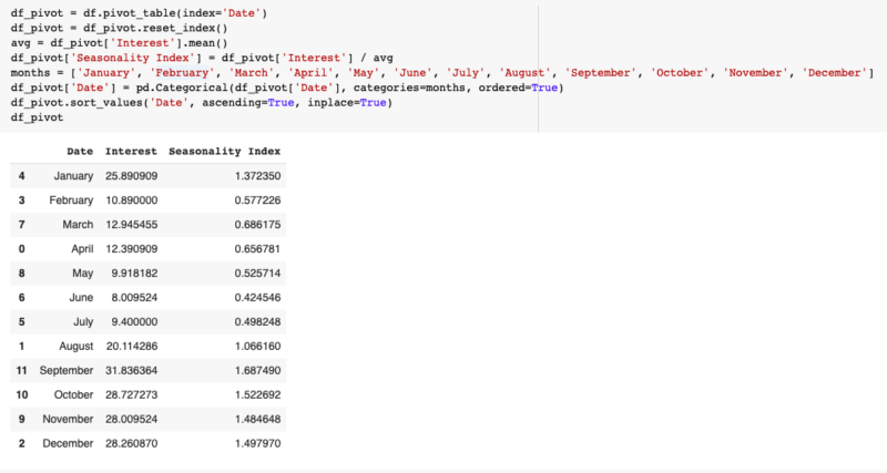
Now, the final step in creating our seasonality index is to group the data by month and convert it to an index. This can be done by calculating the average interest throughout the year and dividing each month’s interest by the average interest.

This can be done in Pandas by calculating the mean of the Interest and then dividing each item in the series by the mean.
Step 3: Put It All Together in Google Sheets
Now that we have our seasonality index, it’s time to put it to work. This could be done in Python but since we’ll want to be able to change some of the inputs to our projection model, I think it’s easiest to use Google Sheets or Excel.
I have created this Google Sheet as an example.
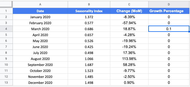
We’ll first create a spreadsheet with our seasonality index and calculate the percentage change from month to month.
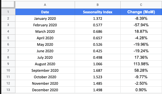
We calculate month over month percentage change using the following function:
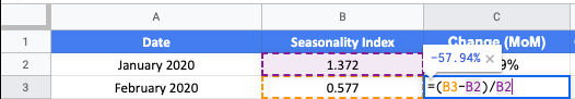
In order to calculate the percentage for January, you’ll need to modify the function. Calculate percent change using the formula below.

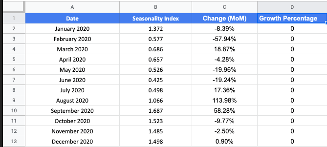
We’ll also create a column for Growth Percentage. This is what we’ll use to model the growth driven by the projects we plan to complete this year. Set the values to 0 for now, we’ll come back to this later.
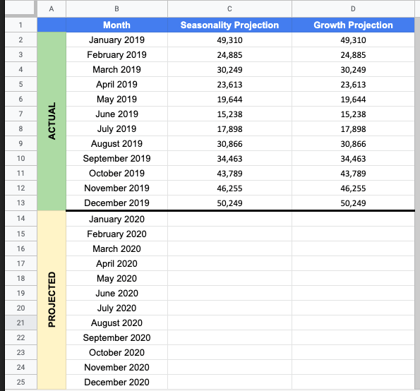
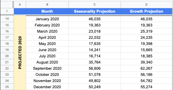
In a new tab, we’ll add traffic from the past year by month in two columns: Seasonality Projection and Growth Projection. We’ll also continue the Month column to include this year.
Projecting traffic using seasonality
Now, we’ll use our seasonality index to project monthly traffic based on December’s traffic. This calculation uses the growth percentage in the Seasonality tab in our sheet as follows:

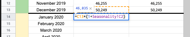
Then, we can drag this function down so it fills in the rest of the months in the year.
If we take the sum of this year, we’ll have our projected annual traffic for 2020.

Projecting traffic using growth and seasonality
Next, we’ll add the expected growth from the projects we hope to complete this year. Repeat the steps above but also add the Growth Percentage column from the Seasonality tab.
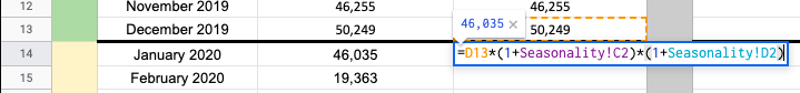
Let’s imagine we have a project in March that we expect will lead to a 10% increase in traffic. We navigate to the Seasonality tab and change the value in the Growth Percentage column for March from 0 to 0.1.
This will now update the Growth Projections in the Traffic tab to reflect a 10% increase in March. Compare the values for March in the Seasonality column to the values in the Growth column. Also, notice that the values for each month after March have increased as well. That is the value of this model.
Now we can plot this difference on a time series chart.

We can also calculate the total projected traffic for 2020 given the impact of this project and compare it to the projected traffic based on seasonality. That gives you the total value of completing this project in March.
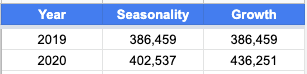
Based on this model and the traffic data, completing this project in March would lead to an increase of 33,714 visits to the site. That can then be quantified even further. Let’s imagine our conversion rate is around 2% for SEO traffic. That means this change would bring in an additional 674 conversions this year. Let’s also imagine our AOV (average order value) is $80. That means this change could drive a revenue increase of $53,920 this year. This tool lays the groundwork for making these types of calculations. Is the math absolutely perfect? Not by a long shot but it at least gives you some means of prioritization and helps you tell the story of why the items on your SEO roadmap are important.
Contributing authors are invited to create content for Search Engine Land and are chosen for their expertise and contribution to the search community. Our contributors work under the oversight of the editorial staff and contributions are checked for quality and relevance to our readers. The opinions they express are their own.
Related stories
About the author