How to use RStudio to create traffic forecasting models
Learn the basics of producing time series forecasts in RStudio from your Google Search Console click data.
There is a lot of fervor in the SEO industry for Python right now.
It is a comparably easier programming language to learn and has become accessible to the SEO community through guides and blogs.
But if you want to learn a new language for analyzing and visualizing your search data, consider looking into R.
This article covers the basics of how you can produce time series forecasts in RStudio from your Google Search Console click data.
But first, what is R?
R is “a language and environment for statistical computing and graphics,” according to The R Project for Statistical Computing.
R isn’t new and has been around since 1993. Still, learning some of the basics of R – including how to interact with Google’s various APIs – can be advantageous for SEOs.
If you want to pick up R as a new language, good courses to learn from are:
- Data Analysis with R Programming (Offered by Google)
- R Programming (Offered by Johns Hopkins University)
But if you grasp the basics and want to learn data visualization fundamentals in R, I recommend Coursera’s guided project, Application of Data Analysis in Business with R Programming.
And then you also need to install:
- R (through the Comprehensive R Archive Network).
- Posit’s RStudio integrated development environment (IDE) – which is to R as PyCharm is to Python.
What follows are the steps for creating traffic forecasting models in RStudio using click data.
Step 1: Prepare the data
The first step is to export your Google Search Console data. You can either do this through the user interface and exporting data as a CSV:

Or, if you want to pull your data via RStudio directly from the Google Search Console API, I recommend you follow this guide from JC Chouinard.
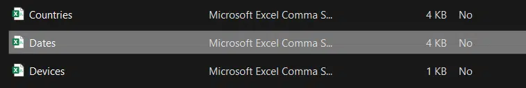
If you do this via the interface, you’ll download a zip file with various CSVs, from which you want the workbook named “Dates”:
Your date range can be from a quarter, six months, or 12 months – all that matters is that you have the values in chronological order, which this export easily produces. (You just need to sort Column A, so the oldest values are at the top.)
Step 2: Plot the time series data in RStudio
Now we need to import and plot our data. To do this, we must first install four packages and then load them.
The first command to run is:
## Install packagesinstall.packages("tidyverse")
install.packages("tsibble")
install.packages("fabletools")
install.packages("bsts")
Followed by:
## Load packageslibrary("tidyverse")
library("tsibble")
library("fabletools")
library("bsts")
You then want to import your data. The only change you need to make to the below command is the file type name (maintaining the CSV extension) in red:
## Read datamdat <- read_csv("example data csv.csv",
col_types = cols(Date = col_date(format = "%d/%m/%Y")))
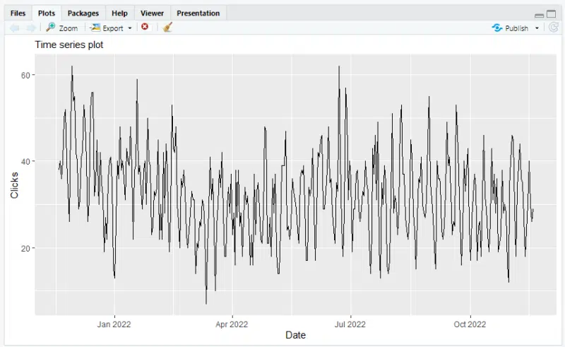
Then the last two commands in plotting your data are to make the time series the object, then to plot the graph itself:
## Make time series objectts_data <- mdat %>%
as_tsibble(index = "Date")
Followed by:
## Make plotautoplot(ts_data) +
labs(x = "Date", subtitle = "Time series plot")
And in your RStudio interface, you will have a time series plot appear:
Step 3: Model and forecast your data in RStudio
At this stage, it’s important to acknowledge that forecasting is not an exact science and relies on several truths and assumptions. These being:
- Assumptions that historical trends and patterns shall continue to replicate with varying degrees over time.
- Forecasting will contain errors and anomalies because your data set (your real-world clicks data) will contain anomalies that could be construed as errors.
- Forecasts typically revolve around the average, making group forecasts more reliable than running a series of micro-forecasts.
- Shorter-range forecasting is typically more accurate than longer-range forecasting.
With this out of the way, we can begin to model and forecast our traffic data.
For this article, I will visualize our data as a Bayesian Structural Time Series (BSTS) forecast, one of the packages we installed earlier. This graph is used by most forecasting methods.
Most marketers will have seen or at least be familiar with the model as it is commonly used across many industries for forecasting purposes.
The first command we need to run is to make our data fit the BSTS model:
ss <- AddLocalLinearTrend(list(), ts_data$Clicks)
ss <- AddSeasonal(ss, ts_data$Clicks, nseasons = 52)
model1 <- bsts(ts_data$Clicks,
state.specification = ss,
niter = 500)
And then plot the model components:
plot(model1, "comp")
And now we can visualize one- and two-year forecasts.
Going back to the previously mentioned general forecasting rules, the further into the future you forecast, the less accurate it becomes. Thus, I stick to two years when doing this.
And as BSTS considers an upper and lower bound, it also becomes pretty pointless past a certain point.
The below command will produce a one-year future BSTS forecast for your data:
# 1-year
pred1 <- predict(model1, horizon = 365)
plot(pred1, plot.original = 200)
And you’ll return a graph like this:
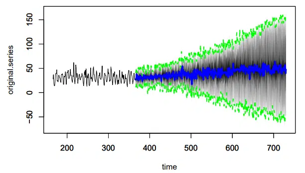
To produce a two-year forecasting graph from your data, you want to run the below command:
pred2 <- predict(model1, horizon = 365*2)
plot(pred2, plot.original = 365)
And this will produce a graph like this:

As you can see, the upper and lower bounds in the one-year forecast had a range of -50 to +150, whereas the 2-year forecast has -200 to +600.
The further into the future you forecast, the greater this range becomes and, in my opinion, the less useful the forecast becomes.
Contributing authors are invited to create content for Search Engine Land and are chosen for their expertise and contribution to the search community. Our contributors work under the oversight of the editorial staff and contributions are checked for quality and relevance to our readers. Search Engine Land is owned by Semrush. Contributor was not asked to make any direct or indirect mentions of Semrush. The opinions they express are their own.